Summary:  Some observations about new major trends and directions in data science drawn from the Strata+Hadoop conference in San Jose last week.

I’m fresh off my annual field trip to the Strata+Hadoop conference in San Jose last week.  This is always exciting, enervating, and exhausting but it remains the single best place to pick up on what’s changing in our profession.

This conference is on a world tour with four more stops before repeating next year.  The New York show is supposed to be a little bigger (hard to imagine) but the San Jose show is closest to our intellectual birthplace.  After all this is the place where to call yourself a nerd would be regarded as a humble brag.

I’ll try to briefly share the major themes and changes I found this year and will write later in more depth about some of these.

End of the Era of Hadoop

From the time it went open source in 2007 Hadoop and its related technologies have been profound drivers of the growth of data science.  Doug Cutting remains one of the three Strata conference chairs.  However, we all know that Hadoop/MapReduce has made its mark but that it’s no longer cutting edge.  In fact we know that Apache Spark has eclipsed Hadoop and it would be fair to say that Spark was last year’s big news.

To put a stake in it, O’Reilly announced at this year’s Strata+Hadoop that the conference would henceforth be known as the Strata Data Conference.  So farewell age of Hadoop.

Artificial Intelligence

I am as jaded as the next guy and maybe a little more so at the over hyped furor around AI.  As I walked the conference floor I felt compelled to challenge any vendor with the temerity to put AI in their descriptors.

Actually there was very little of this at the show.  AI tends to be most over hyped when we’re talking about apps but Strata+Hadoop is more about tools than apps.  There were two or three vendors that I thought had applied the AI frosting a little thick but there were a few others where the label was appropriate and the capabilities pretty interesting.  More about these good guys later.

In the learning program there were again two or three sessions aimed at AI use cases in business and these were uniformly well reasoned.  Specifically that means acknowledging that this is in its infancy and while you should keep an eye on it, investing now would be speculative at best.

The Cambrian Explosion in Deep Learning

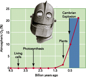One of our general session speakers used this phrase to describe the hockey-stick like growth we’ve been experiencing in Deep Learning and AI in general.  The original use of the phrase is credited to Gill Pratt, the DARPA Program Manager who oversaw the DARPA Robotics Challenge.

If you remember a little about your earth history, we trundled along with one-celled creatures for billions of years until about a half-a-billion years ago when, at the beginning of the Cambrian period, life diversified in a way that can truly be characterized as an explosion.  Academic theory is that very small changes like the evolution of sight organs so changed the playing field that the exploitation of this new capability drove the development of additional capabilities that – you know – resulted in us.

So while data scientists are a little cautious to talk about the wonders of artificial intelligence, they are very enthusiastic in talking about the new capabilities presented by Deep Learning.  This may seem a little paradoxical but I invite you to think about it this way.

Robust AI is the accumulated capabilities of speech, text, NLP, image processing, robotics, knowledge recovery, and several other human-like capabilities that at this point are very early in development and not at all well or easily integrated.

Deep Learning however is a group of tools that we are applying to develop these capabilities, including Convolutional Neural Nets, Recurrent Neural Nets, Generative Adversarial Neural Nets, and Reinforcement Learning to name the most popular.  All of these are subsets of Deep Learning and all are accessed through the newly emerging Deep Learning platforms like TensorFlow, MXNet, Theano, Torch, and several others.

Like all platform battles, the winner who gains the most users will be the next IoS, Android, or Windows.  Right now it appears Google’s TensorFlow is in the lead and there were at least four or five program sessions, some of them full-day, that were oversubscribed providing both general guidance as well as hands-on training in TensorFlow.  So while the buzz around AI was appropriately subdued, the enthusiasm for learning about TensorFlow was in full flower.  The emergence of Deep Learning platforms may be the slight evolutionary change that triggers the explosion of AI.

Platform Convergence

In the beginning you could pick a portion of the data science workflow and build a successful business there.  Many of today’s largest companies got their start this way.  Not anymore.  Now everybody wants to be an end-to-end platform from data source to the deployment of models and other forms of exploitation.  He with the most users will win and once adopted the pain of switching will be high.  The same dynamic that continues to make enterprise ERP systems so sticky – it’s too painful to switch.

We’ve seen in the last years analytic platforms like SAS and SPSS add full data access and blending capability.  We’ve seen blending platforms like Alteryx extend into analytics and visualization.  So here are two new and rather unexpected additions to the full spectrum platform game:

Cloudera announces its own Data Science Workbench with capabilities in R, Python, and Scala.

Intel (yes Intel?) who just paid $15 Billion for Mobileye to seize its place in the self-driving car space is rolling out two data science platforms, Saffron and Nirvana, one aimed at IoT and the other at deep learning.

DataOps and Data Engineers

As recently as a year or so ago the term ‘data scientist’ applied to someone doing predictive analytics as well as the person you would turn to to implement Spark or a data lake.  Thankfully over not too long a period we have come to differentiate Data Scientists from Data Engineers and acknowledge their special skill set that blends traditional CS skills with the new disciplines needed to store, extract, and utilize data for data scientists.

Now that this differentiation is a little clearer, we see a parallel rise in a new category of tools and platforms best described as DataOps.  Philosophically similar to DevOps, DataOps tools and platforms are aimed at regularizing and simplifying the tasks of Data Engineers, particularly as it applies to repetitive tasks that may need to be repeated dozens or even hundreds of times for different data sources and different data destinations.  Two new companies, both startups, Nexla, and Data Kitchen take a fairly narrow but deep view.  Others like Qubole are laying claim to this area by better defining capabilities within their existing platforms.

Emerging Productivity Enhancements for Data Scientists

We may think the business world is populated by companies with just a few (if any) data scientists working together and for the most part we’d be right.  However, this is not the market most vendors at Strata are interested in.  They are pursuing wallet share among the Global 8000.  That’s 8000 companies with more than $1 Billion in revenue and assuredly 100% commitment to predictive analytics.

I haven’t seen any specific data but an informal poll of vendors says these companies employee from 20 to several hundred data scientists each.  When you have that many data scientists in one place you have to start thinking about efficiency and productivity.  And there’s a major theme for this year – productivity enhancements for data scientists.

The list of vendors with this focus is too long for this article and DataOps just above is part of this.  Here are just a few mentions of notable companies and their approach.

DataRobot:  We reviewed DataRobot a year ago when it looked like predictive analytics was about to be fully automated and data scientists unemployed by 2025.  That was a little premature.  However, DataRobot has found a foothold by dramatically speeding up model development.  This is one-click-to-model.  Their platform cleans data, does feature engineering and identification, runs thousands of potential models/hyper parameter combinations in parallel, and deploys champion models in a fraction of the time it would take a team of data scientists.

SqlStream:  Deploy a blazing fast stream processing system in a fraction of the time and with a fraction of the compute resources distros like Spark require.  Make it so easy to manage that very little is needed of data engineers, and make it easy to change the logic and models within the stream without a team of data scientists.

Bansai:  TensorFlow is complex and tough to learn.  Bansai is introducing a higher level language that looks a lot like Python but manipulates deep learning algorithms in all the major deep learning platforms.  Their initial target is reinforcement learning for robotics and the payoff is to solve the shortage of deep learning-qualified data scientists that are a bottleneck for development.

Qubole:  Makes it easy to almost instantly establish a big data repository and begin analytics.  You can’t completely replace data engineers but you can dramatically increase the number of data scientists each engineer can support with this SaaS implementation.

Emergence of the Data Science Appliance

Similar to productivity enhancements but aimed at business users who want solutions without necessarily needing to know the underlying data science are a group of offerings that intentionally hide the data science and focus on the business problem.

Anodot:  Delivers a sophisticated anomaly detection system that looks at all your streaming data and decides both what’s anomalous and what’s important.  This is catching on among ecommerce vendors and digital enterprises, some of whom have reportedly thrown out their internally developed anomaly detectors in favor of Anodot’s offering.

GeoStrategies:  This company uses GIS data for site location and market identification and penetration studies.  Lots of sophisticated platforms can do that too but GeoStrategies goes out of its way to hide the data science in favor of a UI that’s very intuitive for their business users.

Women in Data Science

Finally, my unscientific tally was that about 20% of attendees and a slightly higher percentage of presenters were women.  This may not be representative of our profession as a whole as folks who attend these conferences may have different profiles than the whole industry.  Still, while we might wish this was more like 50/50 I thought participation by our female members was a reasonably strong showing.

About the author:  Bill Vorhies is Editorial Director for Data Science Central and has practiced as a data scientist and commercial predictive modeler since 2001.

This problem appeared as an assignment in the online coursera course Convolution Neural Networks by Prof Andrew Ng, (deeplearing.ai).  The description of the problem is taken straightway from the assignment.

In this assignment, we shall:

• Implement the neural style transfer algorithm
• Generate novel artistic images using our algorithm

Most of the algorithms we’ve studied optimize a cost function to get a set of parameter values. In Neural Style Transfer, we  shall optimize a cost function to get pixel values!

Problem Statement

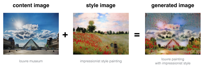
Neural Style Transfer (NST) is one of the most fun techniques in deep learning. As seen below, it merges two images, namely,

1. a “content” image (C) and
2. a “style” image (S),

to create a “generated” image (G). The generated image G combines the “content” of the image C with the “style” of image S.

In this example, we are going to generate an image of the Louvre museum in Paris (content image C), mixed with a painting by Claude Monet, a leader of the impressionist movement (style image S).

Let’s see how we can do this.

Transfer Learning

Neural Style Transfer (NST) uses a previously trained convolutional network, and builds on top of that. The idea of using a network trained on a different task and applying it to a new task is called transfer learning.

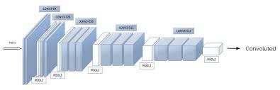
Following the original NST paper, we shall use the VGG network. Specifically, we’ll use VGG-19, a 19-layer version of the VGG network. This model has already been trained on the very large ImageNet database, and thus has learned to recognize a variety of low level features (at the earlier layers) and high level features (at the deeper layers). The following figure shows how a VGG-19 convolution neural net looks like, without the last fully-connected (FC) layers.

We run the following code to load parameters from the pre-trained VGG-19 model serialized in a matlab file. This takes a few seconds.
model = load_vgg_model(“imagenet-vgg-verydeep-19.mat”)
import pprint
pprint.pprint(model)

{‘avgpool1’: <tf.Tensor ‘AvgPool_5:0’ shape=(1, 150, 200, 64) dtype=float32>,
‘avgpool2’: <tf.Tensor ‘AvgPool_6:0’ shape=(1, 75, 100, 128) dtype=float32>,
‘avgpool3’: <tf.Tensor ‘AvgPool_7:0’ shape=(1, 38, 50, 256) dtype=float32>,
‘avgpool4’: <tf.Tensor ‘AvgPool_8:0’ shape=(1, 19, 25, 512) dtype=float32>,
‘avgpool5’: <tf.Tensor ‘AvgPool_9:0’ shape=(1, 10, 13, 512) dtype=float32>,
‘conv1_1’: <tf.Tensor ‘Relu_16:0’ shape=(1, 300, 400, 64) dtype=float32>,
‘conv1_2’: <tf.Tensor ‘Relu_17:0’ shape=(1, 300, 400, 64) dtype=float32>,
‘conv2_1’: <tf.Tensor ‘Relu_18:0’ shape=(1, 150, 200, 128) dtype=float32>,
‘conv2_2’: <tf.Tensor ‘Relu_19:0’ shape=(1, 150, 200, 128) dtype=float32>,
‘conv3_1’: <tf.Tensor ‘Relu_20:0’ shape=(1, 75, 100, 256) dtype=float32>,
‘conv3_2’: <tf.Tensor ‘Relu_21:0’ shape=(1, 75, 100, 256) dtype=float32>,
‘conv3_3’: <tf.Tensor ‘Relu_22:0’ shape=(1, 75, 100, 256) dtype=float32>,
‘conv3_4’: <tf.Tensor ‘Relu_23:0’ shape=(1, 75, 100, 256) dtype=float32>,
‘conv4_1’: <tf.Tensor ‘Relu_24:0’ shape=(1, 38, 50, 512) dtype=float32>,
‘conv4_2’: <tf.Tensor ‘Relu_25:0’ shape=(1, 38, 50, 512) dtype=float32>,
‘conv4_3’: <tf.Tensor ‘Relu_26:0’ shape=(1, 38, 50, 512) dtype=float32>,
‘conv4_4’: <tf.Tensor ‘Relu_27:0’ shape=(1, 38, 50, 512) dtype=float32>,
‘conv5_1’: <tf.Tensor ‘Relu_28:0’ shape=(1, 19, 25, 512) dtype=float32>,
‘conv5_2’: <tf.Tensor ‘Relu_29:0’ shape=(1, 19, 25, 512) dtype=float32>,
‘conv5_3’: <tf.Tensor ‘Relu_30:0’ shape=(1, 19, 25, 512) dtype=float32>,
‘conv5_4’: <tf.Tensor ‘Relu_31:0’ shape=(1, 19, 25, 512) dtype=float32>,
‘input’: <tensorflow.python.ops.variables.Variable object at 0x7f7a5bf8f7f0>}
The next figure shows the content image (C) – the Louvre museum’s pyramid surrounded by old Paris buildings, against a sunny sky with a few clouds.

For the above content image, the activation outputs from the convolution layers are visualized in the next few figures.

How to ensure that the generated image G matches the content of the image C?

As we know, the earlier (shallower) layers of a ConvNet tend to detect lower-level features such as edges and simple textures, and the later (deeper) layers tend to detect higher-level features such as more complex textures as well as object classes.

We would like the “generated” image G to have similar content as the input image C. Suppose we have chosen some layer’s activations to represent the content of an image. In practice, we shall get the most visually pleasing results if we choose a layer in the middle of the network – neither too shallow nor too deep.

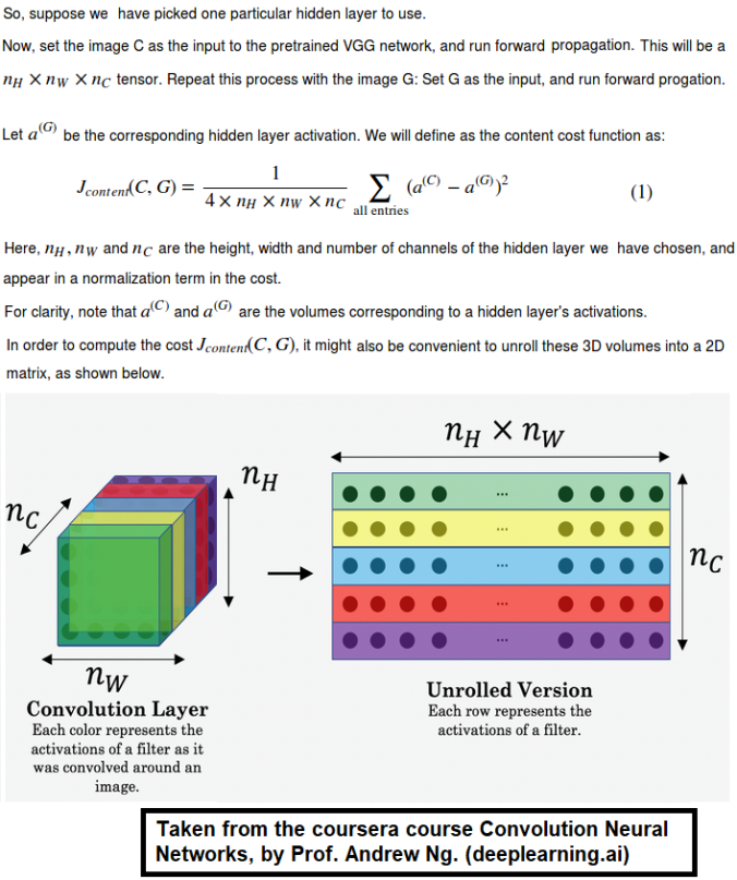
First we need to compute the “content cost” using TensorFlow.

• The content cost takes a hidden layer activation of the neural network, and measures how different a(C) and a(G) are.
• When we minimize the content cost later, this will help make sure G
  has similar content as C.

def compute_content_cost(a_C, a_G):
“””
Computes the content cost

Arguments:
a_C — tensor of dimension (1, n_H, n_W, n_C), hidden layer activations representing content of the image C
a_G — tensor of dimension (1, n_H, n_W, n_C), hidden layer activations representing content of the image G

Returns:
J_content — scalar that we need to compute using equation 1 above.
“””

# Retrieve dimensions from a_G
m, n_H, n_W, n_C = a_G.get_shape().as_list()

# Reshape a_C and a_G
a_C_unrolled = tf.reshape(tf.transpose(a_C), (m, n_H * n_W, n_C))
a_G_unrolled = tf.reshape(tf.transpose(a_G), (m, n_H * n_W, n_C))

# compute the cost with tensorflow
J_content = tf.reduce_sum((a_C_unrolled – a_G_unrolled)**2 / (4.* n_H * n_W *
n_C))

return J_content

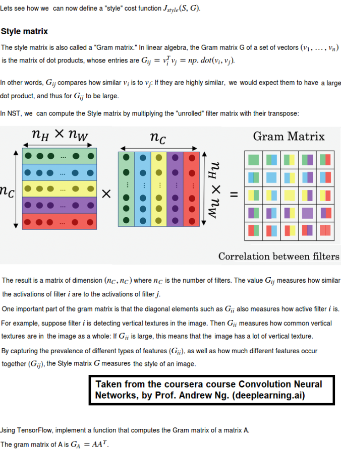
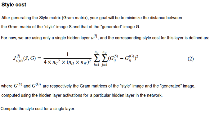
Computing the style cost

For our running example, we will use the following style image (S). This painting was painted in the style of impressionism, by  Claude Monet .

def gram_matrix(A):
“””
Argument:
A — matrix of shape (n_C, n_H*n_W)

Returns:
GA — Gram matrix of A, of shape (n_C, n_C)
“””

GA = tf.matmul(A, tf.transpose(A))
return GA

def compute_layer_style_cost(a_S, a_G):
“””
Arguments:
a_S — tensor of dimension (1, n_H, n_W, n_C), hidden layer activations representing style of the image S
a_G — tensor of dimension (1, n_H, n_W, n_C), hidden layer activations representing style of the image G

Returns:
J_style_layer — tensor representing a scalar value, style cost defined above by equation (2)
“””

# Retrieve dimensions from a_G
m, n_H, n_W, n_C = a_G.get_shape().as_list()

# Reshape the images to have them of shape (n_C, n_H*n_W)
a_S = tf.reshape(tf.transpose(a_S), (n_C, n_H * n_W))
a_G = tf.reshape(tf.transpose(a_G), (n_C, n_H * n_W))

# Computing gram_matrices for both images S and G (≈2 lines)
GS = gram_matrix(a_S)
GG = gram_matrix(a_G)

# Computing the loss
J_style_layer = tf.reduce_sum((GS – GG)**2 / (4.* (n_H * n_W * n_C)**2))

return J_style_layer

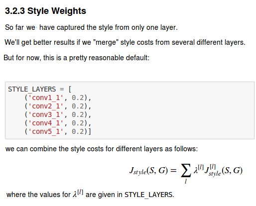
• The style of an image can be represented using the Gram matrix of a hiddenlayer’s activations. However, we get even better results combining this representation from multiple different layers. This is in contrast to the content representation, where usually using just a single hidden layer is sufficient.
• Minimizing the style cost will cause the image G to follow the style of the image S.

Defining the total cost to optimize

Finally, let’s create and implement a cost function that minimizes both the style and the content cost. The formula is:

https://sandipanweb.files.wordpress.com/2018/01/12.png?w=150&h=16 150w” sizes=”(max-width: 456px) 100vw, 456px” />
def total_cost(J_content, J_style, alpha = 10, beta = 40):
“””
Computes the total cost function

Arguments:
J_content — content cost coded above
J_style — style cost coded above
alpha — hyperparameter weighting the importance of the content cost
beta — hyperparameter weighting the importance of the style cost

Returns:
J — total cost as defined by the formula above.
“””

J = alpha * J_content + beta * J_style
return J

• The total cost is a linear combination of the content cost J_content(C,G) and the style cost J_style(S,G).
• α and β are hyperparameters that control the relative weighting between content and style. (we have used values 10 and 40 respectively for α and β).

Solving the optimization problem

Finally, let’s put everything together to implement Neural Style Transfer!

Here’s what the program will have to do:

• Create an Interactive Session
• Load the content image
• Load the style image
• Randomly initialize the image to be generated
• Load the VGG19 model
• Build the TensorFlow graph:
  • Run the content image through the VGG19 model and compute the content cost.
  • Run the style image through the VGG19 model and compute the style cost
    Compute the total cost.
  • Define the optimizer and the learning rate.
• Initialize the TensorFlow graph and run it for a large number of iterations (we have used 200 iterations), updating the generated image at every step.

Let’s first load, reshape, and normalize our “content” image (the Louvre museum picture) and “style” image (Claude Monet’s painting).

Now, we initialize the “generated” image as a noisy image created from the content_image. By initializing the pixels of the generated image to be mostly noise but still slightly correlated with the content image, this will help the content of the “generated” image more rapidly match the content of the “content” image. The following figure shows the noisy image:

Next, let’s load the pre-trained VGG-19 model.

To get the program to compute the content cost, we will now assign a_C and a_G to be the appropriate hidden layer activations. We will use layer conv4_2 to compute the content cost. We need to do the following:

• Assign the content image to be the input to the VGG model.
• Set a_C to be the tensor giving the hidden layer activation for layer “conv4_2”.
• Set a_G to be the tensor giving the hidden layer activation for the same layer.
• Compute the content cost using a_C and a_G.

Next, we need to compute the style cost and compute the total cost J by taking a linear combination of the two. Use alpha = 10 and beta = 40.

Then we are going to  set up the Adam optimizer in TensorFlow, using a learning rate of 2.0.

Finally, we need to initialize the variables of the tensorflow graph, assign the input image (initial generated image) as the input of the VGG19 model and runs the model to minimize the total cost J for a large number of iterations.

Results

The following figures show the generated images (G) with different content (C) and style images (S) at different iterations in the optimization process.

Content

Style (Claud Monet’s The Poppy Field near Argenteuil)

Generated

Content

Style

Generated

Content

Style

Generated

Content

Style (Van Gogh’s The Starry Night)

Generated

Content

Style

Generated

Content (Victoria Memorial Hall)

Style (Van Gogh’s The Starry Night)

Generated

Content (Taj Mahal)

Style (Van Gogh’s Starry Night Over the Rhone)

Generated

Content (me)

Style (Van Gogh’s Irises)

Generated

In this article, I clarify the various roles of the data scientist, and how data science compares and overlaps with related fields such as machine learning, deep learning, AI, statistics, IoT, operations research, and applied mathematics. As data science is a broad discipline, I start by describing the different types of data scientists that one may encounter in any business setting: you might even discover that you are a data scientist yourself, without knowing it. As in any scientific discipline, data scientists may borrow techniques from related disciplines, though we have developed our own arsenal, especially techniques and algorithms to handle very large unstructured data sets in automated ways, even without human interactions, to perform transactions in real-time or to make predictions.

1. Different Types of Data Scientists

Recently (August 2016)  Ajit Jaokar discussed Type A (Analytics) versus Type B (Builder) data scientist:

• The Type A Data Scientist can code well enough to work with data but is not necessarily an expert. The Type A data scientist may be an expert in experimental design, forecasting, modelling, statistical inference, or other things typically taught in statistics departments. Generally speaking though, the work product of a data scientist is not “p-values and confidence intervals” as academic statistics sometimes seems to suggest (and as it sometimes is for traditional statisticians working in the pharmaceutical industry, for example). At Google, Type A Data Scientists are known variously as Statistician, Quantitative Analyst, Decision Support Engineering Analyst, or Data Scientist, and probably a few more.

• Type B Data Scientist: The B is for Building. Type B Data Scientists share some statistical background with Type A, but they are also very strong coders and may be trained software engineers. The Type B Data Scientist is mainly interested in using data “in production.” They build models which interact with users, often serving recommendations (products, people you may know, ads, movies, search results). 

I also wrote about the ABCD’s of business processes optimization where D stands for data science, C for computer science, B for business science, and A for analytics science. Data science may or may not involve coding or mathematical practice, as you can read in my article on low-level versus high-level data science. In a startup, data scientists generally wear several hats, such as executive, data miner, data engineer or architect, researcher, statistician, modeler (as in predictive modeling) or developer.

While the data scientist is generally portrayed as a coder experienced in R, Python, SQL, Hadoop and statistics, this is just the tip of the iceberg, made popular by data camps focusing on teaching some elements of data science. But just like a lab technician can call herself a physicist, the real physicist is much more than that, and her domains of expertise are varied: astronomy, mathematical physics, nuclear physics (which is borderline chemistry), mechanics, electrical engineering, signal processing (also a sub-field of data science) and many more. The same can be said about data scientists: fields are as varied as bioinformatics, information technology, simulations and quality control, computational finance, epidemiology, industrial engineering, and even number theory.

In my case, over the last 10 years, I specialized in machine-to-machine and device-to-device communications, developing systems to automatically process large data sets, to perform automated transactions: for instance, purchasing Internet traffic or automatically generating content. It implies developing algorithms that work with unstructured data, and it is at the intersection of AI (artificial intelligence,) IoT (Internet of things,) and data science. This is referred  to as deep data science. It is relatively math-free, and it involves relatively little coding (mostly API’s), but it is quite data-intensive (including building data systems) and based on brand new statistical technology designed specifically for this context.

Prior to that, I worked on credit card fraud detection in real time. Earlier in my career (circa 1990) I worked on image remote sensing technology, among other things to identify patterns (or shapes or features, for instance lakes) in satellite images and to perform image segmentation: at that time my research was labeled as computational statistics, but the people doing the exact same thing in the computer science department next door in my home university, called their research artificial intelligence. Today, it would be called data science or artificial intelligence, the sub-domains being signal processing, computer vision or IoT.

Also, data scientists can be found anywhere in the lifecycle of data science projects, at the data gathering stage, or the data exploratory stage, all the way up to statistical modeling and maintaining existing systems.

2. Machine Learning versus Deep Learning

Before digging deeper into the link between data science and machine learning, let’s briefly discuss machine learning and deep learning. Machine learning is a set of algorithms that train on a data set to make predictions or take actions in order to optimize some systems. For instance, supervised classification algorithms are used to classify potential clients into good or bad prospects, for loan purposes, based on historical data. The techniques involved, for a given task (e.g. supervised clustering), are varied: naive Bayes, SVM, neural nets, ensembles, association rules, decision trees, logistic regression, or a combination of many. For a detailed list of algorithms, click here. For a list of machine learning problems, click here.

All of this is a subset of data science. When these algorithms are automated, as in automated piloting or driver-less cars, it is called AI, and more specifically, deep learning. Click here for another article comparing machine learning with deep learning. If the data collected comes from sensors and if it is transmitted via the Internet, then it is machine learning or data science or deep learning applied to IoT.

Some people have a different definition for deep learning. They consider deep learning as neural networks (a machine learning technique) with a deeper layer. The question was asked on Quora recently, and below is a more detailed explanation (source: Quora)

• AI (Artificial intelligence) is a subfield of computer science, that was created in the 1960s, and it was (is) concerned with solving tasks that are easy for humans, but hard for computers. In particular, a so-called Strong AI would be a system that can do anything a human can (perhaps without purely physical things). This is fairly generic, and includes all kinds of tasks, such as planning, moving around in the world, recognizing objects and sounds, speaking, translating, performing social or business transactions, creative work (making art or poetry), etc.

• NLP (Natural language processing) is simply the part of AI that has to do with language (usually written).

• Machine learning is concerned with one aspect of this: given some AI problem that can be described in discrete terms (e.g. out of a particular set of actions, which one is the right one), and given a lot of information about the world, figure out what is the “correct” action, without having the programmer program it in. Typically some outside process is needed to judge whether the action was correct or not. In mathematical terms, it’s a function: you feed in some input, and you want it to to produce the right output, so the whole problem is simply to build a model of this mathematical function in some automatic way. To draw a distinction with AI, if I can write a very clever program that has human-like behavior, it can be AI, but unless its parameters are automatically learned from data, it’s not machine learning.

• Deep learning is one kind of machine learning that’s very popular now. It involves a particular kind of mathematical model that can be thought of as a composition of simple blocks (function composition) of a certain type, and where some of these blocks can be adjusted to better predict the final outcome.

What is the difference between machine learning and statistics?

This article tries to answer the question. The author writes that statistics is machine learning with confidence intervals for the quantities being predicted or estimated. I tend to disagree, as I have built engineer-friendly confidence intervals that don’t require any mathematical or statistical knowledge.

3. Data Science versus Machine Learning

Machine learning and statistics are part of data science. The word learning in machine learning means that the algorithms depend on some data, used as a training set, to fine-tune some model or algorithm parameters. This encompasses many techniques such as regression, naive Bayes or supervised clustering. But not all techniques fit in this category. For instance, unsupervised clustering – a statistical and data science technique – aims at detecting clusters and cluster structures without any a-priori knowledge or training set to help the classification algorithm. A human being is needed to label the clusters found. Some techniques are hybrid, such as semi-supervised classification. Some pattern detection or density estimation techniques fit in this category.

Data science is much more than machine learning though. Data, in data science, may or may not come from a machine or mechanical process (survey data could be manually collected, clinical trials involve a specific type of small data)  and it might have nothing to do with learning as I have just discussed. But the main difference is the fact that data science covers the whole spectrum of data processing, not just the algorithmic or statistical aspects. In particular, data science also covers

• data integration
• distributed architecture
• automating machine learning
• data visualization
• dashboards and BI
• data engineering
• deployment in production mode
• automated, data-driven decisions

Of course, in many organisations, data scientists focus on only one part of this process.