


Deep Learning & Art: Neural Style Transfer – An Implementation with Tensorflow in Python
Posted on August 12th, 2018
Posted by Sandipan Dey on January 2, 2018 at 1:00pm
View Blog
This problem appeared as an assignment in the online coursera course Convolution Neural Networks by Prof Andrew Ng, (deeplearing.ai). The description of the problem is taken straightway from the assignment.
In this assignment, we shall:
- Implement the neural style transfer algorithm
- Generate novel artistic images using our algorithm
Most of the algorithms we’ve studied optimize a cost function to get a set of parameter values. In Neural Style Transfer, we shall optimize a cost function to get pixel values!
Problem Statement
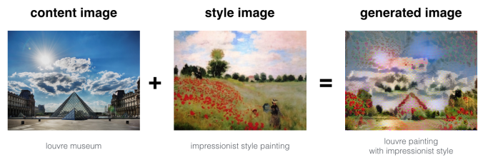
Neural Style Transfer (NST) is one of the most fun techniques in deep learning. As seen below, it merges two images, namely,
- a “content” image (C) and
- a “style” image (S),
to create a “generated” image (G). The generated image G combines the “content” of the image C with the “style” of image S.
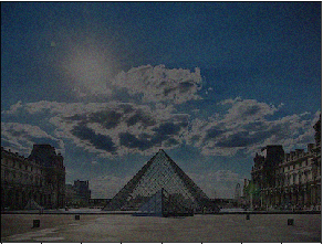
In this example, we are going to generate an image of the Louvre museum in Paris (content image C), mixed with a painting by Claude Monet, a leader of the impressionist movement (style image S).
Let’s see how we can do this.
Transfer Learning
Neural Style Transfer (NST) uses a previously trained convolutional network, and builds on top of that. The idea of using a network trained on a different task and applying it to a new task is called transfer learning.
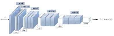
Following the original NST paper, we shall use the VGG network. Specifically, we’ll use VGG-19, a 19-layer version of the VGG network. This model has already been trained on the very large ImageNet database, and thus has learned to recognize a variety of low level features (at the earlier layers) and high level features (at the deeper layers). The following figure shows how a VGG-19 convolution neural net looks like, without the last fully-connected (FC) layers.
We run the following code to load parameters from the pre-trained VGG-19 model serialized in a matlab file. This takes a few seconds.
model = load_vgg_model(“imagenet-vgg-verydeep-19.mat”)
import pprint
pprint.pprint(model)
{‘avgpool1’: <tf.Tensor ‘AvgPool_5:0’ shape=(1, 150, 200, 64) dtype=float32>,
‘avgpool2’: <tf.Tensor ‘AvgPool_6:0’ shape=(1, 75, 100, 128) dtype=float32>,
‘avgpool3’: <tf.Tensor ‘AvgPool_7:0’ shape=(1, 38, 50, 256) dtype=float32>,
‘avgpool4’: <tf.Tensor ‘AvgPool_8:0’ shape=(1, 19, 25, 512) dtype=float32>,
‘avgpool5’: <tf.Tensor ‘AvgPool_9:0’ shape=(1, 10, 13, 512) dtype=float32>,
‘conv1_1’: <tf.Tensor ‘Relu_16:0’ shape=(1, 300, 400, 64) dtype=float32>,
‘conv1_2’: <tf.Tensor ‘Relu_17:0’ shape=(1, 300, 400, 64) dtype=float32>,
‘conv2_1’: <tf.Tensor ‘Relu_18:0’ shape=(1, 150, 200, 128) dtype=float32>,
‘conv2_2’: <tf.Tensor ‘Relu_19:0’ shape=(1, 150, 200, 128) dtype=float32>,
‘conv3_1’: <tf.Tensor ‘Relu_20:0’ shape=(1, 75, 100, 256) dtype=float32>,
‘conv3_2’: <tf.Tensor ‘Relu_21:0’ shape=(1, 75, 100, 256) dtype=float32>,
‘conv3_3’: <tf.Tensor ‘Relu_22:0’ shape=(1, 75, 100, 256) dtype=float32>,
‘conv3_4’: <tf.Tensor ‘Relu_23:0’ shape=(1, 75, 100, 256) dtype=float32>,
‘conv4_1’: <tf.Tensor ‘Relu_24:0’ shape=(1, 38, 50, 512) dtype=float32>,
‘conv4_2’: <tf.Tensor ‘Relu_25:0’ shape=(1, 38, 50, 512) dtype=float32>,
‘conv4_3’: <tf.Tensor ‘Relu_26:0’ shape=(1, 38, 50, 512) dtype=float32>,
‘conv4_4’: <tf.Tensor ‘Relu_27:0’ shape=(1, 38, 50, 512) dtype=float32>,
‘conv5_1’: <tf.Tensor ‘Relu_28:0’ shape=(1, 19, 25, 512) dtype=float32>,
‘conv5_2’: <tf.Tensor ‘Relu_29:0’ shape=(1, 19, 25, 512) dtype=float32>,
‘conv5_3’: <tf.Tensor ‘Relu_30:0’ shape=(1, 19, 25, 512) dtype=float32>,
‘conv5_4’: <tf.Tensor ‘Relu_31:0’ shape=(1, 19, 25, 512) dtype=float32>,
‘input’: <tensorflow.python.ops.variables.Variable object at 0x7f7a5bf8f7f0>}
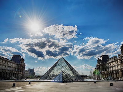
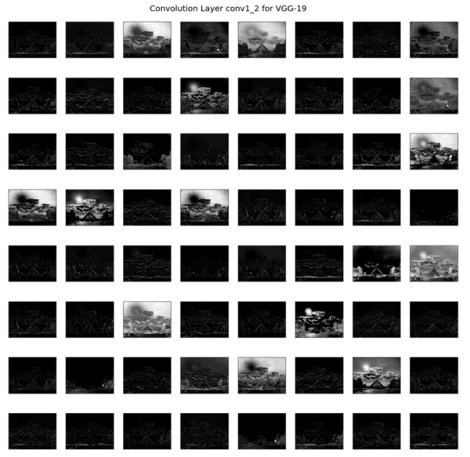
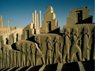
The next figure shows the content image (C) – the Louvre museum’s pyramid surrounded by old Paris buildings, against a sunny sky with a few clouds.
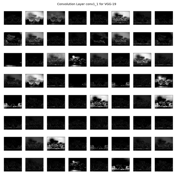
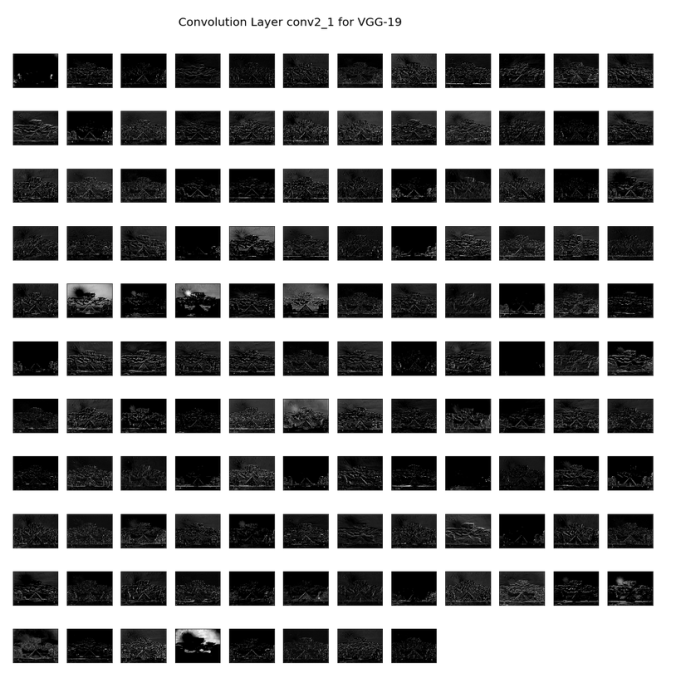
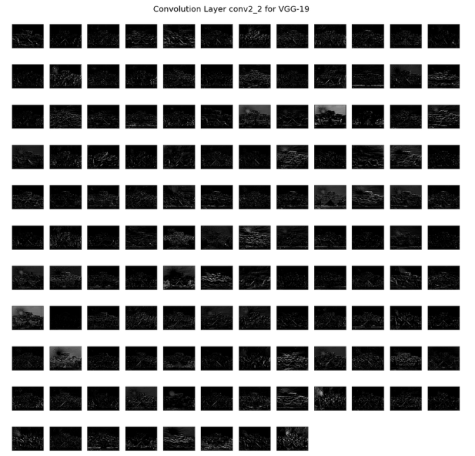
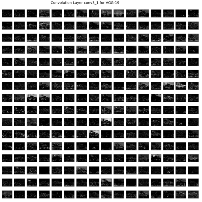
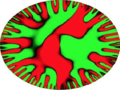
For the above content image, the activation outputs from the convolution layers are visualized in the next few figures.
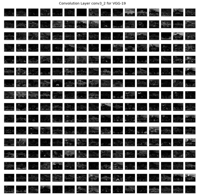
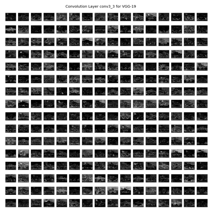
How to ensure that the generated image G matches the content of the image C?
As we know, the earlier (shallower) layers of a ConvNet tend to detect lower-level features such as edges and simple textures, and the later (deeper) layers tend to detect higher-level features such as more complex textures as well as object classes.
We would like the “generated” image G to have similar content as the input image C. Suppose we have chosen some layer’s activations to represent the content of an image. In practice, we shall get the most visually pleasing results if we choose a layer in the middle of the network – neither too shallow nor too deep.
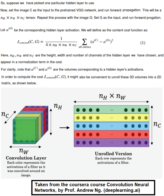
First we need to compute the “content cost” using TensorFlow.
- The content cost takes a hidden layer activation of the neural network, and measures how different a(C) and a(G) are.
- When we minimize the content cost later, this will help make sure G
has similar content as C.
def compute_content_cost(a_C, a_G):
“””
Computes the content cost
Arguments:
a_C — tensor of dimension (1, n_H, n_W, n_C), hidden layer activations representing content of the image C
a_G — tensor of dimension (1, n_H, n_W, n_C), hidden layer activations representing content of the image G
Returns:
J_content — scalar that we need to compute using equation 1 above.
“””
# Retrieve dimensions from a_G
m, n_H, n_W, n_C = a_G.get_shape().as_list()
# Reshape a_C and a_G
a_C_unrolled = tf.reshape(tf.transpose(a_C), (m, n_H * n_W, n_C))
a_G_unrolled = tf.reshape(tf.transpose(a_G), (m, n_H * n_W, n_C))
# compute the cost with tensorflow
J_content = tf.reduce_sum((a_C_unrolled – a_G_unrolled)**2 / (4.* n_H * n_W *
n_C))
return J_content
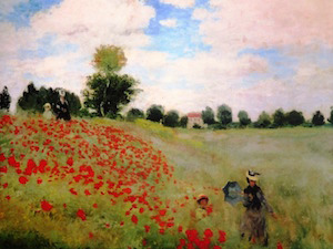
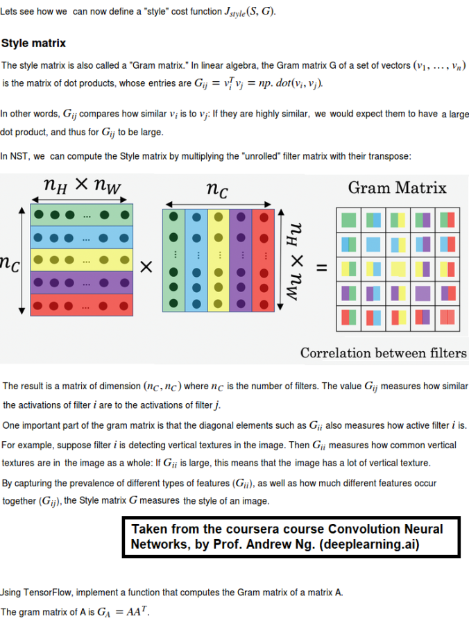
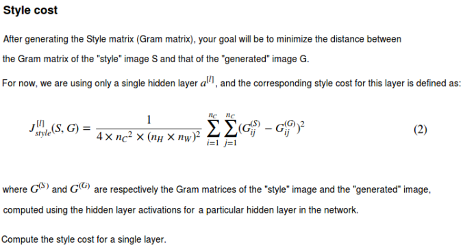
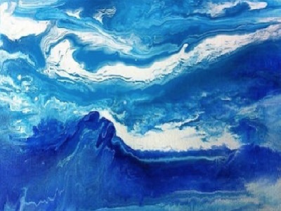
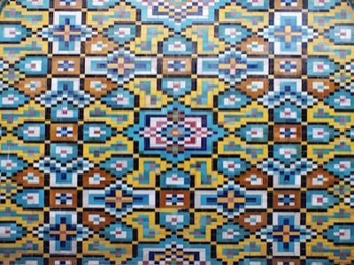
Computing the style cost
For our running example, we will use the following style image (S). This painting was painted in the style of impressionism, by Claude Monet .
def gram_matrix(A):
“””
Argument:
A — matrix of shape (n_C, n_H*n_W)
Returns:
GA — Gram matrix of A, of shape (n_C, n_C)
“””
GA = tf.matmul(A, tf.transpose(A))
return GA
def compute_layer_style_cost(a_S, a_G):
“””
Arguments:
a_S — tensor of dimension (1, n_H, n_W, n_C), hidden layer activations representing style of the image S
a_G — tensor of dimension (1, n_H, n_W, n_C), hidden layer activations representing style of the image G
Returns:
J_style_layer — tensor representing a scalar value, style cost defined above by equation (2)
“””
# Retrieve dimensions from a_G
m, n_H, n_W, n_C = a_G.get_shape().as_list()
# Reshape the images to have them of shape (n_C, n_H*n_W)
a_S = tf.reshape(tf.transpose(a_S), (n_C, n_H * n_W))
a_G = tf.reshape(tf.transpose(a_G), (n_C, n_H * n_W))
# Computing gram_matrices for both images S and G (≈2 lines)
GS = gram_matrix(a_S)
GG = gram_matrix(a_G)
# Computing the loss
J_style_layer = tf.reduce_sum((GS – GG)**2 / (4.* (n_H * n_W * n_C)**2))
return J_style_layer
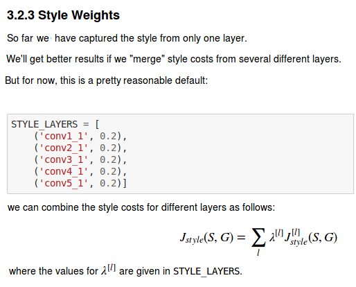
- The style of an image can be represented using the Gram matrix of a hiddenlayer’s activations. However, we get even better results combining this representation from multiple different layers. This is in contrast to the content representation, where usually using just a single hidden layer is sufficient.
- Minimizing the style cost will cause the image G to follow the style of the image S.
Defining the total cost to optimize
Finally, let’s create and implement a cost function that minimizes both the style and the content cost. The formula is:
 https://sandipanweb.files.wordpress.com/2018/01/12.png?w=150&h=16 150w” sizes=”(max-width: 456px) 100vw, 456px” />
def total_cost(J_content, J_style, alpha = 10, beta = 40):
“””
Computes the total cost function
Arguments:
J_content — content cost coded above
J_style — style cost coded above
alpha — hyperparameter weighting the importance of the content cost
beta — hyperparameter weighting the importance of the style cost
Returns:
J — total cost as defined by the formula above.
“””
J = alpha * J_content + beta * J_style
return J
- The total cost is a linear combination of the content cost J_content(C,G) and the style cost J_style(S,G).
- α and β are hyperparameters that control the relative weighting between content and style. (we have used values 10 and 40 respectively for α and β).
Solving the optimization problem
Finally, let’s put everything together to implement Neural Style Transfer!
Here’s what the program will have to do:
- Create an Interactive Session
- Load the content image
- Load the style image
- Randomly initialize the image to be generated
- Load the VGG19 model
- Build the TensorFlow graph:
- Run the content image through the VGG19 model and compute the content cost.
- Run the style image through the VGG19 model and compute the style cost
Compute the total cost. - Define the optimizer and the learning rate.
- Initialize the TensorFlow graph and run it for a large number of iterations (we have used 200 iterations), updating the generated image at every step.
Let’s first load, reshape, and normalize our “content” image (the Louvre museum picture) and “style” image (Claude Monet’s painting).
Now, we initialize the “generated” image as a noisy image created from the content_image. By initializing the pixels of the generated image to be mostly noise but still slightly correlated with the content image, this will help the content of the “generated” image more rapidly match the content of the “content” image. The following figure shows the noisy image:
Next, let’s load the pre-trained VGG-19 model.
To get the program to compute the content cost, we will now assign a_C and a_G to be the appropriate hidden layer activations. We will use layer conv4_2 to compute the content cost. We need to do the following:
- Assign the content image to be the input to the VGG model.
- Set a_C to be the tensor giving the hidden layer activation for layer “conv4_2”.
- Set a_G to be the tensor giving the hidden layer activation for the same layer.
- Compute the content cost using a_C and a_G.
Next, we need to compute the style cost and compute the total cost J by taking a linear combination of the two. Use alpha = 10 and beta = 40.
Then we are going to set up the Adam optimizer in TensorFlow, using a learning rate of 2.0.
Finally, we need to initialize the variables of the tensorflow graph, assign the input image (initial generated image) as the input of the VGG19 model and runs the model to minimize the total cost J for a large number of iterations.
Results
The following figures show the generated images (G) with different content (C) and style images (S) at different iterations in the optimization process.
Content

Style (Claud Monet’s The Poppy Field near Argenteuil)

Generated
Content
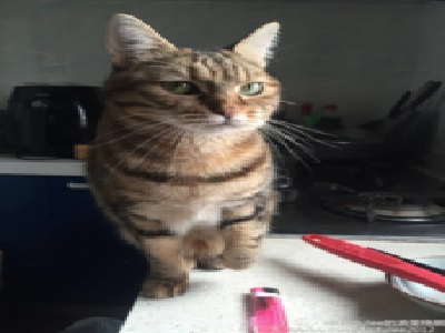
Style
Generated
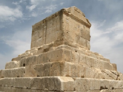
Content
Style
Generated
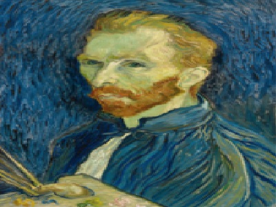
Content
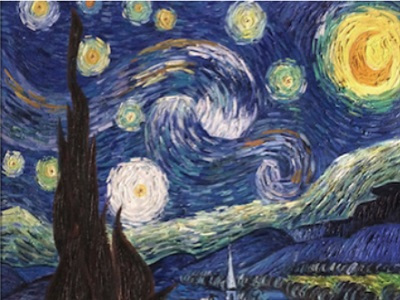
Style (Van Gogh’s The Starry Night)

Generated
Content
Style
Generated
Content (Victoria Memorial Hall)
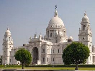
Style (Van Gogh’s The Starry Night)
Generated
Content (Taj Mahal)
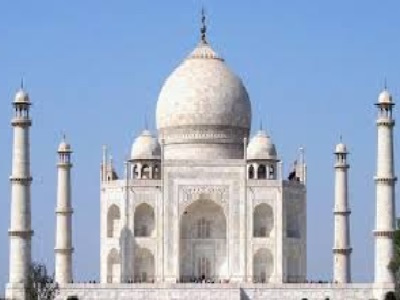
Style (Van Gogh’s Starry Night Over the Rhone)
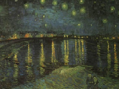
Generated
Content (me)

Style (Van Gogh’s Irises)
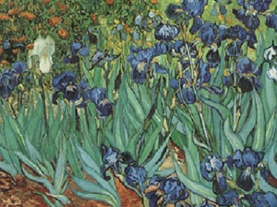
Generated
Content retrieved from: https://www.datasciencecentral.com/profiles/blogs/deep-learning-amp-art-neural-style-transfer-an-implementation.